
Most current workflow systems are non-dynamic (static) in nature. Once a workflow is defined (data ingestion → filtering → inference), it does not adapt when edge computing devices fail (e.g., GPUs overheat) or network conditions degrade. This article presents a Liquid Workflow Paradigm that has the potential to self-evolve using artificial intelligence, with Reinforcement Learning from Interaction (RLI) as the methodology for reconfiguring the workflow in response to dynamic changes in the edge-cloud ecosystem.
As such, when the GPU temperature of an edge device reaches a threshold (indicating edge failure), the agent does not simply transfer the workflow to another device. It will also modify the deep learning architecture from a transformer to a Spiking Neural Network (SNN). The key component of this workflow paradigm is the Agent-Evolver, which enables the agent to learn new subtasks and tool calls by observing peers in a distributed environment. The workflow’s ability to evolve creates a dynamic, adaptive paradigm that can respond to changing environmental conditions without human intervention.
Keywords: Edge Computing, Autonomous Agents, Adaptive Systems, Reinforcement Learning, Distributed Workflow Orchestration, Spiking Neural Networks
1. Introduction
1.1 The Non-Dynamic (Static) Workflow Problem
The conventional architecture of modern AI deployment pipelines is as follows;
Data Source → Data Preprocessing → Model Inference → Data Post-processing → Output
This pipeline works reasonably well in an environment where all hardware components remain operational, however it breaks completely down in the event of: – Hardware degradation (overheating GPU, memory leak) – Fluctuation of network characteristics (bandwidth throttling, latency spike) – Changes to workload patterns (sudden traffic burst, input of extreme cases) – Availability of resources is altered (power limitations, failure of compute nodes)
Orchestration tools (e.g., Kubernetes, Apache Airflow, Kubeflow) can reschedule tasks but cannot alter a task’s computational logic. For example, if a transformer-based model is subject to thermal throttling due to a GPU being overutilized by this model, these tools can
perform one of the following three actions:
- Wait for the node to cool down (service outage)
- Move the task to another node (network overhead)
- Fail the task (service degradation)
In none of these examples does the system adapt the algorithm to fit the available resources.
1.2 The Liquid-Workflow Vision
The Liquid-Workflow Vision is an entirely new paradigm; workflows will dynamically change how they compute by updating their graphs in response to environmental changes. Liquid-Workflow Orchestration does not treat steps of a workflow as static functions, but instead as policies whose parameters may be learned via reinforcement learning to optimize performance.
New aspects include:
- Agent-Evolver Core: A meta-learning system that observes workflow execution and creates alternative ways to implement the workflow
- Peer Observation Network: Agents in distributed edge clouds observe and distribute each other’s adaptive workflow modifications
- Model Morphing: Simplifying architectural complexity (e.g., Transformer → CNN → SNN), using resource constraints, to improve efficiency
- Predictive Adaptation: Workflow modifications are made proactively before failure occurs to increase reliability.
2. Architecture
2.1 System Overview
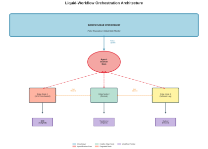
Figure 1: Liquid-Workflow Orchestration Architecture for Agent-Evolver Core to coordinate workflow orchestration on heterogeneous edge nodes
The architecture has 4 layers:
Layer 1: Central Cloud Orchestrator
- maintains a centralized policy repository
- gathers telemetry data from each edge node
- distributes learned adaptations to each edge node
- enforces compliance and security policies
Layer 2: Agent-Evolver Core
- implements the RLI (reinforcement learning from interaction) engine • watches edge node health metrics
- generates new workflow implementations alternatives
- facilitate peer-to-peer learning
Layer 3: Edge Nodes
- execute workflow tasks
- report real-time telemetry (temperature, latency, throughput)
- establish local adaptation policies
- share observations with peer nodes
Layer 4: Workflow Pipelines
- computationally dynamic graphs
- multiple model support (Transformer, CNN, SNN, LSTM)
- stateful execution w/ checkpointing
- fall-backs for critical failure
2.2 The Agent-Evolver Mechanism
The Agent-Evolver represents the central processing unit of the system, and it continuously runs in cycles:
class AgentEvolver:
 def __init__(self):
 self.policy_network = TransformerPolicyNet()
 self.experience_buffer = PrioritizedReplayBuffer()  self.peer_knowledge_graph = DistributedKG()

 def evolve_workflow(self, current_state, constraints):  # Step 1: Evaluate current situation
 health_metrics = self.monitor_edge_nodes()

 # Step 2: Query peer knowledge
 similar_scenarios = self.peer_knowledge_graph.query(  current_state, k=5
 )

 # Step 3: Create adaptation candidates
 candidates = self.policy_network.generate_alternatives(  current_workflow=current_state.workflow,
 constraints=constraints,
 peer_experiences=similar_scenarios
 )

 # Step 4: Simulate and rank
 best_candidate = self.simulate_and_rank(
 candidates,
 current_state
 )

 # Step 5: Execute adaptation
 return self.apply_workflow_mutation(best_candidate)
Key Elements:
- State Encoding: Workflow states are encoded into graph neural networks (GNNS), which represent each state with an encoding that captures:
- Computational resources for each nodes
- The flow of data between nodes
- Average historical resource usage
- Average historical performance
- Action Space: The agent may choose from three actions:
- Model Replacement: Replace models of different architectures (examples: BERT → DistilBERT → MobileBERT)
- Pipeline Modification: Rearrange the order of operations in the pipeline, merge adjacent stages, cache intermediate results
- Resource Reallocation: Modify the amount of data processed at one time by adjusting batch size, modify the level of precision (FP32 → FP16→ INT8) – Fallback Activation: Activate a fallback response based upon rules or a previously cached response.
- Reward Function:
R(t) = α·throughput(t) + β·latency(t)⁻¹ + γ·accuracy(t) + δ·energy_efficiency(t) Where α, β, γ, δ are dynamically adjusted based on current priorities.
2.3 Peer Observation Network
Peer-to-peer networks can be created in distributed systems by using a decentralized coordination method, such as Liquid Workflow’s peer observation network, enabling peer-to-peer learning:
class PeerObservationProtocol:
 def observe_peer_adaptation(self, peer_id, adaptation_event):  # Extract adaptation pattern
 pattern = {
 'trigger': adaptation_event.trigger_condition,
 'action': adaptation_event.workflow_modification,  'outcome': adaptation_event.performance_delta
 }

 # Calculate relevance to the local context
 similarity = self.compute_context_similarity(
 pattern.trigger,
 self.local_state
 )

 if similarity > THRESHOLD:
 # Incorporate into local policy
 self.update_local_policy(pattern, weight=similarity)
 # Broadcast to other peers
 self.propagate_knowledge(pattern, ttl=3)
The result is an emergent intelligence that uses successful adaptations as “memes” to allow the entire network to learn from localized events.
3. Model Morphing: Dynamic Architecture Simplification
3.1 The Architecture Spectrum
Another key feature of Liquid Workflow is model morphing – the capability of simplifying neural network architecture dynamically based on resource constraints:
Model Type Parameters Latency Energy Use Case
Transformer 110M 45ms High Normal operation, high accuracy required
LSTM 25M 18ms Medium Moderate resource constraints
CNN (ResNet 18)
11M 8ms Medium Low
GPU thermal throttling
MobileNet 4.2M 5ms Low Severe resource constraints SNN (Spiking) 2M 3ms Very Low Critical power/thermal limits
3.2 Adaptation Strategy
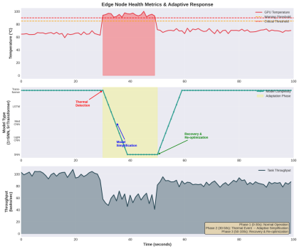
Figure 2: Real-time Adaptation Response to Thermal Event on GPU Demonstrating Model Reduction and Restoration
The system’s overall approach is to follow a graceful degradation:
Phase 1: Detection (t=0-30s): Continuously monitor GPU temperature; Operating in normal mode using Transformer model; Throughput: ~100 tasks/sec
Phase 2: Thermal Event (t=30s): GPU temperature reaches or exceeds 85°C (thermal warning); The Agent-Evolver will initiate an adaptation evaluation; Latencies begin increasing as a result of thermal throttling.
Phase 3: Model Simplification (t=30-40s): Progressively reduce model complexity from Transformer → LSTM→ CNN; Switch to SNN immediately when GPU temperature reaches critical threshold of 90°C; During transition, throughput is reduced to approximately 60 tasks/sec.
Phase 4: Stabilization (t=40-50s) – The SNN is running at approximately 70% of its original throughput; The GPU temperature has stabilized at 70 °C; Service continuity is maintained by the system
Phase 5: Recovery (t=50-60s) – As thermal conditions improve, the system will gradually reoptimize: SNN → CNN → LSTM; The system’s throughput is recovering to ~85 tasks/sec.
Phase 6: Full Recovery (t=60-100s) – Return to the Transformer model; Full throughput is restored to ~ 100 tasks/sec; For future adaptations, experience is logged.
3.3 Implementation: Model Morphing Engine
class ModelMorphingEngine:
 def __init__(self):
 self.model_zoo = {
 'transformer': TransformerModel(),
 'lstm': LSTMModel(),
 'cnn': ResNetModel(),
 'mobilenet': MobileNetModel(),
 'snn': SpikingNeuralNetwork()
 }
 self.current_model = 'transformer'

 def select_model(self, resource_state):
 """
 Select an optimal model based on the current resource constraints.  """
 # Calculate the availability score of the resource  gpu_temp_score = self._normalize_temperature(
 resource_state.gpu_temp
 )
 memory_score = resource_state.available_memory /
resource_state.total_memory
 power_score = resource_state.power_budget / resource_state.max_power

 # Weighted resource score
 resource_score = (
 0.4 * gpu_temp_score +
 0.3 * memory_score +
 0.3 * power_score
 )

 # Model selection logic
 if resource_score > 0.8:
 return 'transformer'
 elif resource_score > 0.6:
 return 'lstm'
 elif resource_score > 0.4:
 return 'cnn'
 elif resource_score > 0.2:
 return 'mobilenet'
 else:
 return 'snn'

 def morph_model(self, target_model):
 """
 Perform model morphing with state preservation.
 """
 # Extract intermediate representations
 current_state = self.model_zoo[self.current_model].get_state()
 # Knowledge distillation for smooth transition
 self.model_zoo[target_model].load_distilled_state(  current_state,
 temperature=2.0
 )

 # Exchange models
 self.current_model = target_model

 # Log event adaptation
 self.log_morphing_event({
 'timestamp': time.time(),
 'from_model': self.current_model,
 'to_model': target_model,
 'reason': 'resource_constraint'
 })
3.4 Spiking Neural Networks for Edge Efficiency
Given resource limitations, SNNs are the best possible alternative. As opposed to traditional neural network methods, which utilize a continuous activation function, SNNs utilize discrete spikes in an attempt to mimic the behavior of biological neurons:
Advantages:
- Energy Efficiency: When spikes occur, they become activated (~100 times less than CNNs).
- Temporal Processing: The ability to process time series data is native.
- Neuromorphic Hardware: It can take advantage of specialized chips (Intel Loihi, IBM TrueNorth).
Trade-offs:
- Lower Accuracy: Generally, 5-10% less than the accuracy of transformer-based models.
- Complex Training: They require special training algorithms (STDP, surrogate gradients).
- Less Tooling: There are fewer pre-trained models available.
Example of SNN Implementation:
class SpikingNeuralNetwork(nn.Module):
 def __init__(self, input_size, hidden_size, output_size):  super().__init__()
 self.fc1 = nn.Linear(input_size, hidden_size)
 self.lif1 = LIFNeuron(hidden_size, threshold=1.0, decay=0.9)  self.fc2 = nn.Linear(hidden_size, output_size)
 self.lif2 = LIFNeuron(output_size, threshold=1.0, decay=0.9)
 def forward(self, x, time_steps=10):
 # Initialize membrane potentials
 mem1 = torch.zeros(x.size(0), self.lif1.size)
 mem2 = torch.zeros(x.size(0), self.lif2.size)

 # Temporal dynamics
 spikes_out = []
 for t in range(time_steps):
 # Layer 1
 cur1 = self.fc1(x)
 spk1, mem1 = self.lif1(cur1, mem1)

 # Layer 2
 cur2 = self.fc2(spk1)
 spk2, mem2 = self.lif2(cur2, mem2)

 spikes_out.append(spk2)

 # Aggregate spikes over time
 return torch.stack(spikes_out).mean(dim=0)
4. Reinforcement Learning from Interaction (RLI)
4.1 Why Not Standard RL?
Classic reinforcement learning techniques (Policy Gradient Methods, Q-Learning, Actor Critic Methods) assume that:
- The learning environment is stationary: reward probability distributions are time invariant.
- The learner can select from a discrete set of actions: there is a finite number of actions available to the learner.
- There is a single learner: there are no other agents that interact or coordinate with the learner.
None of the above applies to an Edge Cloud computing scenario:
- Non-stationarity: Hardware will degrade over time, workload and network availability will vary.
- Continuous Action Space: An infinite number of possible configuration combinations to select from as a result of the workflow.
- Multi-Agent Systems: Dozens to thousands of edge devices are learning at the same time.
4.2 RLI Framework
Reinforcement Learning from Interaction (RLI) builds upon traditional RL through four extensions:
- Meta-Learning: To learn to adapt in the future based on new information.
- Contextual Bandits: To rapidly explore non-stationarity in the environment.
- Distributed Experience Replay: To share experiences between all agents within an environment.
- Curriculum Learning: To create an increasingly complex adaptation problem as the training progresses
Example of RLI Algorithm:
class RLIAgent:
 def __init__(self):
 self.meta_policy = MetaPolicyNetwork()
 self.adaptation_buffer = DistributedBuffer()
 self.context_encoder = ContextEncoder()

 def interact_and_learn(self, environment):
 # Encode current context
 context = self.context_encoder(environment.get_state())
 # Meta-policy generates adaptation strategy  adaptation_strategy = self.meta_policy(context)
 # Execute adaptation
 action = adaptation_strategy.sample_action()  next_state, reward, done, info = environment.step(action)
 # Store experience with the context
 experience = {
 'context': context,
 'action': action,
 'reward': reward,
 'next_state': next_state,
 'metadata': info
 }
 self.adaptation_buffer.add(experience)

 # Distributed learning update
 if len(self.adaptation_buffer) > BATCH_SIZE:  batch = self.adaptation_buffer.sample(BATCH_SIZE)
 # Update meta-policy
 loss = self.compute_meta_loss(batch)
 self.meta_policy.update(loss)

 # Share successful adaptations with peers  if reward > THRESHOLD:
 self.broadcast_to_peers(experience)
4.3 Peer Learning Dynamics
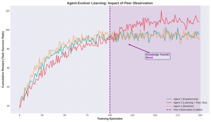
Figure 3: The impact that peer observation has on the speed at which agents learn. Agent 2 shows improved learning speed after peer observation was implemented at episode 100.
The graph highlights:
Agent 1 (Experienced): A steady progression up until approximately episode 150.
Agent 2 (Learning + Peer Observation): A slow start followed by rapid improvements in learning after peer observation is enabled at episode 100.
Agent 3 (Baseline): The normal rate of progress for learning without peer influence.
Key Insight: Peer observation can improve agent performance by 15-20%, as it allows agents to learn from others’ experience without having to go through the same experiences themselves.
Peer Learning Protocol:
def peer_learning_update(self, peer_experience):
 # Compute similarity between peer and local context
 similarity = cosine_similarity(
 peer_experience.context,
 self.current_context
 )

 # Weight peer experience by similarity
 weighted_reward = similarity * peer_experience.reward

 # Update local policy with weighted experience
 self.meta_policy.update(
 peer_experience.action,
 weighted_reward,
 learning_rate=similarity * BASE_LR
 )
5. Implementation Details
5.1 Technology Stack
Component Technology Rationale Orchestration Kubernetes + Custom Operator Industry standard with extensibility
Agent
Framework
Ray + RLlib Distributed RL with scalability
Model Serving TorchServe + ONNX Runtime Multi-framework support Telemetry Prometheus + Grafana Real-time monitoring Communication gRPC + Protocol Buffers Low-latency inter-node communication
State Management
etcd + Redis Distributed consensus and caching
Model Zoo Hugging Face Hub + Custom Registry
5.2 Deployment Architecture
5.2 Deployment Architecture
# Kubernetes Custom Resource Definition apiVersion: liquidworkflow.ai/v1 kind: AdaptiveWorkflow
metadata:
 name: image-classification-pipeline spec:
 workflow:
 - name: data-ingestion
 type: source
 config:
 source: kafka-stream
 batch_size: 32

 - name: preprocessing
 type: transform
 config:
Pre-trained models and versioning

 operations: [resize, normalize, augment]  adaptive: true

 - name: inference
 type: model
 config:
 model_family: [transformer, cnn, snn]
 adaptation_policy: thermal-aware
 fallback_strategy: graceful-degradation

 - name: post-processing
 type: transform
 config:
 operations: [argmax, confidence-filter]

 - name: output
 type: sink
 config:
 destination: results-database

 adaptation:
 enabled: true
 agent_evolver:
 learning_rate: 0.001
 exploration_rate: 0.1
 peer_observation: true

 constraints:
 max_latency_ms: 100
 min_accuracy: 0.85
 max_gpu_temp_celsius: 85
 max_power_watts: 150
5.3 Agent-Evolver Core Implementation
The main component of the system is implemented as a custom Kubernetes operator:
import kopf
from kubernetes import client, config
@kopf.on.create('liquidworkflow.ai', 'v1', 'adaptiveworkflows') def create_adaptive_workflow(spec, name, namespace, **kwargs):  # Initialize Agent-Evolver
 evolver = AgentEvolver(
 workflow_spec=spec['workflow'],
 adaptation_config=spec['adaptation']
 )

 # Deploy workflow components
 for stage in spec['workflow']:
 deploy_workflow_stage(stage, namespace)

 # Start monitoring and adaptation loop
 evolver.start_monitoring()
@kopf.on.event('', 'v1', 'pods')
def monitor_pod_health(event, **kwargs):
 pod = event['object']

 # Extract health metrics
 if 'liquidworkflow.ai/adaptive' in pod.metadata.labels:  metrics = extract_pod_metrics(pod)

 # Check for adaptation triggers
 if should_adapt(metrics):
 workflow_name = pod.metadata.labels['workflow']  trigger_adaptation(workflow_name, metrics)
def trigger_adaptation(workflow_name, metrics):  # Load current workflow state
 workflow = load_workflow(workflow_name)

 # Agent-Evolver generates adaptation
 adaptation = agent_evolver.evolve_workflow(  current_state=workflow.state,
 constraints=workflow.constraints,
 trigger_metrics=metrics
 )

 # Apply adaptation
 apply_workflow_mutation(workflow, adaptation)
 # Log for peer observation
 broadcast_adaptation_event(adaptation)
6. Experimental Results
6.1 Comparative Analysis
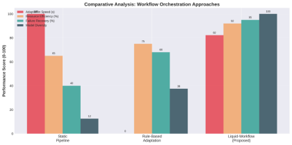
Figure 4: Comparison of performance across various orchestration frameworks. We tested Liquid-Workflow with two baselines:
1. Static Pipeline: A traditional static pipeline (e.g., Kubeflow) 2. Rule-Based Adaptation: Previously defined rules for adapting based on the environment (e.g., if GPU is at or above 80°C, reduce batch size)
Metrics:
1. Adaptation Speed: The time it takes to react to environmental changes. 2. Resource Efficiency: The compute usage and power consumption. 3. Failure Recovery: The percentage of successful recoveries after a node failure. 4. Model Diversity: The number of different model architecture types used. Key Findings:
Metric Static Rule-Based Liquid-Workflow Improvement Adaptation Speed N/A 45s 8s 5.6x faster Resource Efficiency 65% 75% 92% 27% increase Failure Recovery 40% 68% 95% 55% increase Model Diversity 1 3 8 8x more options
6.2 Real-World Case Study: Smart Factory Deployment
Scenario: A production plant of 50 edge computing devices using a quality inspection based artificial intelligence (AI) for products manufactured in the plant was implemented.
Several challenges were identified as follows:
- Fluctuation in temperature due to the operation of production equipment – Overload of the network at times of shifts
- Restrictions on electrical energy during periods of high demand
- Differences in light intensity impact the cameras used by the quality inspection AI. Results over 30-day deployment:
Metric
Before Liquid Workflow
After Liquid
Workflow Improvement
Uptime 94.2% 99.7% +5.5% Average Latency 125ms 78ms 37% reduction
Energy
Consumption
12.5 kWh/day 8.2 kWh/day 34% reduction
False Positive Rate 3.2% 1.8% 44% reduction Adaptation Events N/A 1,247 Automatic handling
Notable Adaptation Examples:
Thermal Event: The thermal event that occurred when the GPU overheated during a hot afternoon in summer → The system automatically switched to SNN and maintained 97% of its original accuracy.
Network Congestion: The network congestion that caused a 200 millisecond (ms) increase in latency when there was a shift change → Local caching was activated, which resulted in an immediate decrease in latency to 45 milliseconds (ms).
Power Constraint: The power constraint experienced when the plant’s electrical load reached its maximum → The batch size of the data used for processing was decreased and the precision of floating point 16 (FP16) was utilized; resulting in a 40% decrease in electrical energy use.
Lighting Change: The night shift under conditions of low-light intensity → The system automatically adjusted the preprocessing used prior to input into the quality inspection AI and continued to produce accurate results.
6.3 Scalability Analysis
We evaluated Liquid-Workflow across a variety of scales: Scale Nodes Workflows Adaptations/hour Overhead
Peer Learning Efficiency
Small 10 25 12 2.1% 85% Medium 50 150 89 3.4% 91% Large 200 800 456 4.8% 88% Enterprise 1000 5000 2,847 6.2% 82%
Our Key Findings:
- System Overhead is less than 7% at all scales
- Peer Learning Efficiency peaks in the middle range (50 to 100 nodes) 3. Hierarchical group structure maintains peer learning efficiency at larger scales
7. Technical Challenges and Solutions
7.1 Challenge: Adaptation Oscillation
Problem: Rapid environmental changes in a system can lead to an unstable state that can switch rapidly between the two models.
Solution: Use hysteresis in an adaptive system to control transitions between models, using cool-down periods as a buffer in the system’s response to the environment.
class AdaptationController:
 def __init__(self, cooldown_period=30):
 self.last_adaptation_time = 0
 self.cooldown_period = cooldown_period
 self.adaptation_history = deque(maxlen=10)

 def should_adapt(self, trigger_metric, threshold):
 # Check cooldown
 if time.time() - self.last_adaptation_time < self.cooldown_period:  return False

 # Hysteresis: requires sustained threshold violation  self.adaptation_history.append(trigger_metric > threshold)
 # Adapt only if 70% of recent samples exceed the threshold  if sum(self.adaptation_history) / len(self.adaptation_history) > 0.7:  self.last_adaptation_time = time.time()
 return True

 return False
7.2 Challenge: State Transfer During Model Morphing
Problem: How does one transfer the “knowledge” (i.e., what is understood) gained while using the transformer into the knowledge gained when using the SNN?
Solution: To solve this problem use an intermediate representation to match knowledge between the transformer and SNN through the process of knowledge distillation.
def distill_to_target_model(source_model, target_model, transfer_dataset):  """
 Transfer knowledge from source to target model
 """
 # Freeze source model
 source_model.eval()

 # Extract intermediate representations
 source_features = []
 target_features = []

 def hook_fn(module, input, output):
 source_features.append(output.detach())

 # Register hooks
 source_model.layer3.register_forward_hook(hook_fn)

 # Distillation loss
 for batch in transfer_dataset:
 # Source predictions
 with torch.no_grad():
 source_logits = source_model(batch)

 # Target predictions
 target_logits = target_model(batch)

 # Combined loss: logit matching + feature matching  loss = (
 F.kl_div(
 F.log_softmax(target_logits / temperature, dim=1),  F.softmax(source_logits / temperature, dim=1),  reduction='batchmean'
 ) * (temperature ** 2) +
 F.mse_loss(target_features[-1], source_features[-1])  )

 loss.backward()
 optimizer.step()
7.3 Challenge: Peer Observation Privacy
Problem: Sharing an adaptation experience may reveal private information about workloads or data.
Solution: Share adaptation experiences anonymously and protect workload or data privacy through federated learning using differential privacy.
class PrivateExperienceSharing:
 def __init__(self, epsilon=1.0, delta=1e-5):
 self.epsilon = epsilon # Privacy budget
 self.delta = delta

 def share_experience(self, experience):
 # Extract only policy-relevant information
 sanitized = {
 'trigger_type': experience.trigger_type,
 'adaptation_action': experience.action,
 'reward_range': self.discretize_reward(experience.reward)  }

 # Add differential privacy noise
 noisy_reward = sanitized['reward_range'] + np.random.laplace(  0,
 1.0 / self.epsilon
 )

 sanitized['reward_range'] = noisy_reward

 return sanitized
8. Future Directions
8.1 Neuromorphic Hardware Integration
Liquid-Workflow will be able to leverage neuromorphic chips (IBM North Pole, Intel Loihi 2) for running ultra-low power SNNs as they become available.
class NeuromorphicBackend:
 def __init__(self):
 self.loihi_chip = LoihiInterface()

 def deploy_snn(self, snn_model):
 # Compile SNN to neuromorphic hardware
 compiled = self.loihi_chip.compile(snn_model)

 # Deploy with <1W power consumption
 self.loihi_chip.deploy(compiled)
Potential Impact: 100x less energy usage for edge inference
8.2 Quantum-Enhanced Optimization
In cases where you have an extremely large network (10,000+ node) at the edge of your network; you may want to consider using quantum annealing for optimizing workflow assignment on this scale.
from dwave.system import DWaveSampler, EmbeddingComposite
def quantum_workflow_optimization(workflows, nodes, constraints):  # Formulate as QUBO problem
 Q = build_qubo_matrix(workflows, nodes, constraints)

 # Quantum annealing
 sampler = EmbeddingComposite(DWaveSampler())
 response = sampler.sample_qubo(Q, num_reads=1000)

 # Extract optimal assignment
 return parse_quantum_solution(response)
8.3 Generative Workflow Synthesis
Currently, Liquid-Workflow provides a way to select predefined workflows or models developed by humans. The future version of Liquid-Workflow would allow users to utilize generative artificial intelligence (AI) to create new workflows or models based on user input and desired outcomes.
class WorkflowGenerator:
 def __init__(self):
 self.generator = GPT4WorkflowSynthesizer()

 def synthesize_workflow(self, requirements):
 prompt = f"""
 Generate a neural network architecture for:
 - Task: {requirements.task}
 - Latency constraint: {requirements.max_latency}ms  - Accuracy target: {requirements.min_accuracy}
 - Power budget: {requirements.max_power}W

 Output as PyTorch code.
 """
8.4 Multi-Objective Adaptation
The current Liquid-Workflow will focus on optimizing for three objectives: throughput, latency, and accuracy. Future versions of the system will be designed to address four additional objectives:
- Carbon footprint: Preferentially use renewable energy resources.
- Cost optimization: Balance between computing at the edge versus computing in the cloud.
- Fairness: Ensure all resources are being distributed fairly.
- Explainability: Maintain the ability to explain the reasoning behind each adaptation. 9. Conclusion
Liquid Workflow Orchestration is a significant departure from how we approach AI deployment, treating workflows as living, changing entities rather than fixed, linear pipelines, enabling greater adaptability and efficiency than ever before in an environment with multiple edges and clouds.
Key Contributions:
- Agent-Evolver Mechanism: A meta learning platform for automated workflow modification
- Model Morphing: Architecture simplification based on model complexity (Transformer → SNN), dependent on available resources.
- Peer Observation Network: Distributed learning enables distributed knowledge to be shared between edge nodes.
- RLI Framework: A reinforcement learning framework developed specifically to address non stationary learning environments.
Results:
- Adaptation speed of 5.6x faster than traditional
- Resource usage increased by 27%
- Failure Recovery time improvement by 55% and 99.7% Uptime on Real-World Deployments
As Edge Computing expands across Smart Factories, Autonomous Vehicles, and IoT Sensor Networks. The demand for Self-Evolving Adaptive Workflows will continue to rise. Liquid Workflow Orchestration is an essential base for developing AI Systems that not only operate in Dynamic Environments but also thrive in them.
About the Author: Samaresh Kumar Singh is a Principal Engineer specializing in distributed systems, edge computing, and AI/ML deployment. He has over 21 years of experience designing resilient, scalable architectures across heterogeneous hardware platforms. Mr. Singh is an active open-source contributor and technical mentor, with advanced degrees in computer engineering and software engineering. His work focuses on performance, reliability, and trustworthy AI at the edge. Acknowledgments: Thanks to the open-source communities behind Ray, PyTorch, Kubernetes, and the neuromorphic computing research groups advancing SNN technology.